
More Information
Submitted: November 11, 2022 | Approved: November 21, 2022 | Published: November 22, 2022
How to cite this article: Cobb KT. Climate change - a review of the mass balance of biogenic and fossil carbon. Arch Biotechnol Biomed. 2022; 6: 014-025.
DOI: 10.29328/journal.abb.1001033
Copyright License: © 2022 Cobb KT. This is an open access article distributed under the Creative Commons Attribution License, which permits unrestricted use, distribution, and reproduction in any medium, provided the original work is properly cited.
Keywords: Keeling Curve; Mass balance; Photosynthesis; Fossil carbon emissions; Biogenic carbon cycle

Climate change - a review of the mass balance of biogenic and fossil carbon
Kirk T Cobb*
4270 Pond View Drive, White Bear Lake, Minnesota 55110, USA
*Address for Correspondence: Kirk T Cobb, 4270 Pond View Drive, White Bear Lake, Minnesota 55110, USA, Email: [email protected]; [email protected]
Trying to understand the causes of climate change can be confusing. On the one hand, methane (CH4) emissions from cattle, and methane emissions from food wastes in landfills, are said to contribute to greenhouse gases (GHGs) that drive climate change. People are working on feed additives for dairy cows to reduce their methane emissions. But, at the same time, cattle manure and food wastes can be fed into anaerobic digesters to convert these organic wastes to biogas; the resulting “renewable methane” or “renewable natural gas” (RNG), can be used in place of fossil natural gas and avoid extra GHG emissions and stop global warming. Can we have it both ways?
Burning gasoline in our cars and trucks generates carbon dioxide (CO2), which is said to contribute to climate change. But more than 8 billion people on planet Earth, breathe in oxygen and exhale carbon dioxide every minute of the day. And so do all the other animals who live on this planet, breathe in oxygen and exhale carbon dioxide. Is our breathing also contributing to climate change, just as the emissions from our automobile tailpipes?
It is time to step back from all the hype, evaluate the various sources of CO2 and CH4 being generated and review the “mass balance” of these gases in our atmosphere. Some of these are part of the natural biogenic carbon cycle and some are simply adding to the overall mass balance. What is driving climate change - excess GHGs from the biogenic carbon cycle, excess emissions from other sources, or both? Let’s take a fresh look at the available data.
(Of course, water vapor also plays a part in the climate change story, as a “positive feedback” effect. As non-condensable GHGs rise in concentration and slightly warm the planet, slightly warming oceans add a bit more water vapor to the story and push the warming up a bit more).
During the past few decades, a great deal of pertinent data has been carefully observed and recorded, by world-class scientists and engineers. This data is available in the public domain and is now easily available on the internet. These data sources come from reputable organizations, such as NASA (National Atmospheric and Space Administration), NOAA (National Oceanic and Atmospheric Administration), USGS (United States Geological Survey) and international organizations such as the “Global Carbon Project” and “Our-World-in-Data”.
How much of the growing concentration of CO2 (and CH4) in our atmosphere can be attributed to out-of-control emissions of biogenic carbon? How much of the CO2 rise can be attributed to fossil fuel emissions: 10%, 50%, 90%, or more?
The available data appear to show that the emissions from burning fossil fuels, more than account for all of the rise of carbon dioxide in our atmosphere during the past 60 years, or longer. In comparison, the biogenic carbon cycle data seem to be very consistent, year after year, decade after decade and have little or no impact on climate change. But, let’s have a closer look at the available data, and let the data speak for itself.
Data in % by volume – convert to % by mass
Much of the important data are available as PPMv (parts per million) by Volume. But, to do an actual “mass balance” these data need to be converted to “mass” data, not “volume” data. The Table 1 is a recent update from the NASA-Earth-Fact-Sheet, as of Sept-2022 and shows carbon dioxide at 415 PPMv. These data will be converted to PPMm (Parts Per Million by mass).
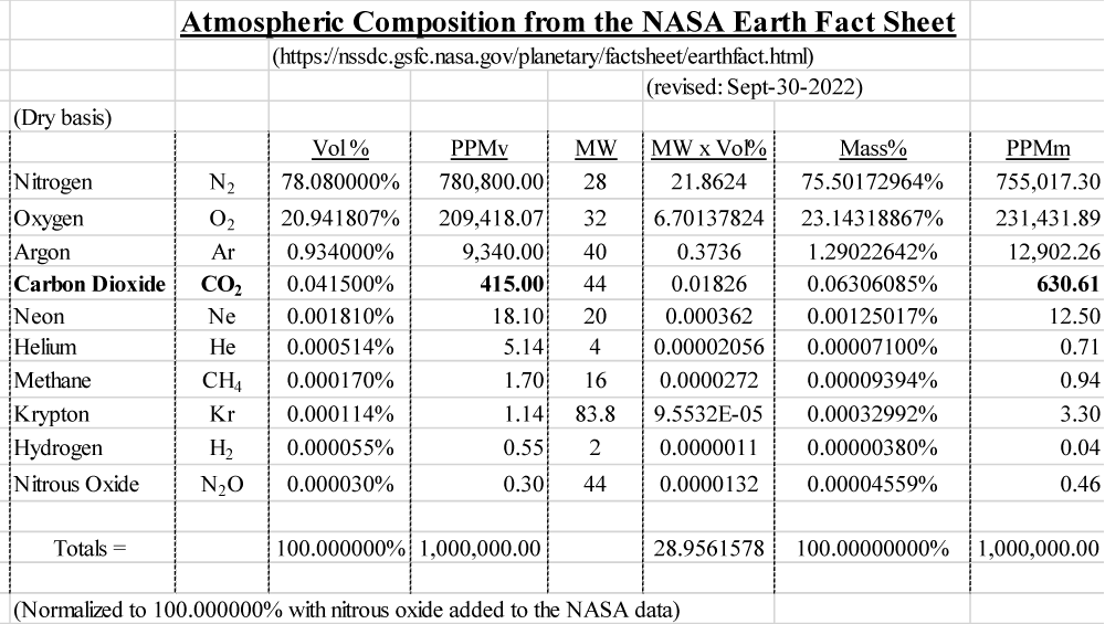
Table 1: Conversion of PPMv to PPMm by Kirk Cobb. [1].
The data above, are available from the NASA website (NASA-Earth-Fact-Sheet) in parts per million by volume. Of course, the volume data are proportional to molar % and have been converted to mass % and PPMm, by applying the molecular weight of each of the gases. Note, that the concentration of CO2 by MASS, is mathematically equivalent to the PPMv x the molecular weight of CO2 (which is 44) and divided by the average molecular weight of the total atmosphere (28.956 – rounded).
So, PPMm of CO2 = PPMv (415) x (44 / 28.956) = 630.61 PPMm. This mathematical relationship will be used later, to convert from volume % to mass %, or PPMv to PPMm.
Another piece of data that may be of interest in this review of available atmospheric data, is a NASA reference to the change in concentration of atmospheric CO2 since 1860. Again, this data set was expressed in PPM by volume (PPMv), so the data have been converted to PPM by mass (PPMm) (Graph 1) (Table 2).
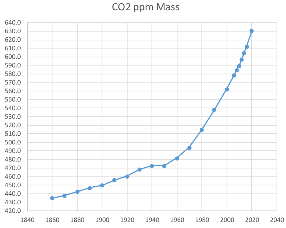
Graph 1: Note – the “2020” data, above, were added to this NASA data from 1860 to 2016.
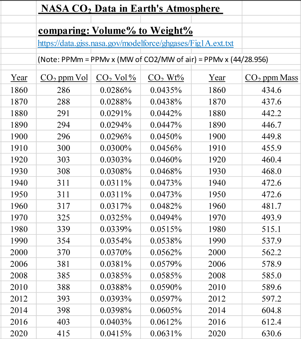
Table 2: [2].
Note that from 1860 to 1960, CO2 increased from ~ 430 to 480 PPMm = 50/100 = 0.5 ppm/year. Then, from 1960 to 2020, CO2 increased from 480 to 630 PPMm; 150/60 = 2.5 ppm/year = a 5-fold rise in rate.
Total mass of earth’s atmosphere
In order the do any sort of mass balance regarding Earth’s atmosphere, an estimate of the total mass of the atmosphere is needed. The mass of Earth’s atmosphere can be determined simply by multiplying atmospheric pressure x the surface area of the planet.
Atmospheric pressure [3] = 14.7 pounds/sq-inch = 2,116.8 lbs/sq-foot = 10,335 kilograms/sq-meter. (The task to confirm these unit conversions, has been left to the reader.) On a grander scale, Atmospheric Pressure (at sea level) = 10,335,000 metric-tonnes/sq-kilometer. (Again, the task to confirm these unit conversions, has been left to the reader.)
Some basic geometry of planet earth [4]
Earth’s diameter = 12,742 kilometers (= 7,917.5 miles). This is based on the NASA-Earth-Fact-Sheet, with a mean radius of Earth = 6,371 kilometers, so diameter = 12,742 kilometers. Since Earth is essentially a sphere, the area of a sphere = PI x D^2. So, Earth’s surface area = PI x D^2 = 510,064,472 square kilometers; let’s just “round” this number to 510,000,000 square kilometers.
The mass of earth’s atmosphere [5]
So, an estimate of the total mass of Earth’s Atmosphere = 10,335,000 MT/sq-kilometer x 510,000,000 sq-kilometers = 5,270,850,000,000,000 Metric-Tonnes. That is a big number! A “Giga-Tonne” (GT) = one-Billion Tonnes, so the mass of Earth’s Atmosphere can be expressed as 5,270,850 GT. This estimate of atmospheric mass may be a bit high since it assumes that it is all based on sea level; in fact, some of Earth’s “land” surface is above sea level, thus displacing a small fraction of the atmosphere.
The NASA Fact Sheet and Wikipedia website note the mass of Earth’s atmosphere to be 5.15 x 10¹⁸ Kilograms. This is within 2.4% of the above estimate. So, from this point forward, the Earth’s atmospheric mass will be assumed to agree with the NASA figure of 5,150,000 GT [5].
How much CO2 is in our atmosphere?
Now that we know the total tonnage of the atmosphere and the “mass percentage” of each component, we can estimate the total tonnage of each gas in our atmosphere. Of particular interest is the rise of Carbon Dioxide, since it is changing so rapidly. As of 2020, according to the data reviewed above, the total mass of our atmosphere is 5,150,000 GT (gigatonnes) x the weight% of carbon dioxide 630.6 PPMm = 3,248 GT (gigatonnes) of carbon dioxide is in our atmosphere. We can also estimate the rate at which CO2 has been increasing during the past few decades. But, before looking at the rate of rise, there is one more very important piece of information that needs to be included in this review of atmospheric data. This data is also available online, from the NOAA website. It is called the “Keeling Curve”.
To honor this 20th Century distinguished scientist, a bit of his biography is included here.
The keeling curve: (The information below is sourced from the online references, as noted) [6].
Charles David Keeling was born in Scranton, Pennsylvania, on April 20, 1928. He completed a Ph.D. in chemistry from Northwestern University in 1954 and was a postdoctoral fellow in geochemistry at the California Institute of Technology from 1953-56. Charles David Keeling was affiliated with Scripps Institution of Oceanography, University of California, San Diego, from 1956 until his death in 2005 [6].
Charles David Keeling, of Scripps Institution of Oceanography at UC San Diego, was the first person to make frequent regular measurements of atmospheric CO2 concentrations on Mauna Loa, Hawaii from March 1958 onwards. Keeling was ……able to maintain operations at the Mauna Loa Observatory until he died in 2005. In Charles Keeling’s honor, these important CO2 measurements have continued, after his death, to the present day (2022)…..by scientists at the Scripps Institute of Oceanography, University of California, San Diego and the National Oceanic and Atmospheric Administration (NOAA). According to Naomi Oreskes, Professor of History of Science at Harvard University, the Keeling curve is one of the most important scientific works of the 20th century. Within a few years of measurements, the Mauna Loa record changed the notion of the atmospheric CO2 increase from a matter of theory to a matter of fact. This was an achievement of tremendous social and political importance, and within the scientific community… the Mauna Loa record, or "Keeling Curve", as it is sometimes called, has become a standard icon symbolizing the impact of humans on the planet. In 2002, President George W. Bush selected Keeling to receive the National Medal of Science, the nation's highest award for lifetime achievement in scientific research [7] (Graph 2).
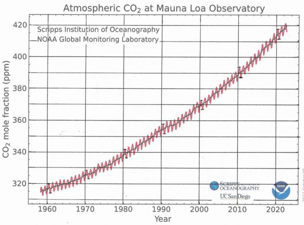
Graph 2: The “Keeling Curve.
Here is the most recent Keeling Curve, published by the “NOAA Global Monitoring Laboratory” as of October 5, 2022.
The Keeling Curve shows two important aspects of CO2 concentrations in the atmosphere. First, note the seasonal oscillation of the CO2 concentrations each year. These will be viewed, and discussed, in more detail in a moment. The other obvious trend is the continuous rise of CO2 concentrations from year to year. This will also be discussed in more detail (Graph 3).
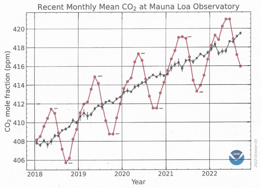
Graph 3: [8].
The chart above, Graph 3 [8], is a recent excerpt (Oct-5-2022) of the above Keeling Curve, showing in more detail, the monthly average concentrations of CO2 from 2018 through 2021(and part of 2022) - follow the red dots. When studying this graph, several items become obvious. Each year, the peak CO2 concentration occurs in May and the lowest concentration occurs in September. From the high to low concentration each year, there is a very repeatable, seasonal oscillation of concentration, of ~ 6 PPMv.
What is causing this oscillation? It is due to the summer activity of photosynthesis in the Northern Hemisphere. Another perspective on this seasonal trend is offered below. These simple 2-dimensional graphs of planet Earth, clearly note that most of the land masses of Earth are in the Northern Hemisphere.
World geometry facts Note the location of the equator, passing through northern South America and southern Africa, in the charts [9].
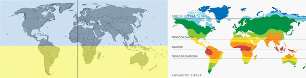
The Northern Hemisphere has much more land than the Southern Hemisphere. About 68% of the world's land area is in the Northern Hemisphere while the Southern Hemisphere contains ~32% of the world’s land area.
Water covers 70.78% of Earth's surface. The land covers 29.22% of Earth’s surface. Earth’s Diameter = 12,742 kilometers (= 7,918 miles). Earth’s total spherical surface area = PI x Diam^2 = 510,000,000 square kilometers. Earth’s Land area = 149,000,000 sq-kilometers;
Earth’s Water area = 361,000,000 sq-kilometers;
Southern Hemisphere Land = ~ 47,680,000 sq-kilometers;
Northern Hemisphere Land = ~ 101,320,000 sq-kilometers [9].
The CO2 seasonal cycle data shown on the Keeling Curve, clearly demonstrate the dominance of photosynthesis and the biogenic carbon cycle in the Northern Hemisphere, compared to the much smaller land mass of the Southern Hemisphere. Charles David Keeling’s data, which he began to measure and record in 1958, are simply astounding! In fact, the seasonal oscillation actually shows the differential between the opposing photosynthetic northern and southern cycles, but with the northern cycle being the more dominant effect.
Refer, again, back to Graph 2, the total Keeling Curve, from 1958 to 2022. From decade to decade, the data in Table 3, have been inferred from Graph 2.
Graph 3: [8].
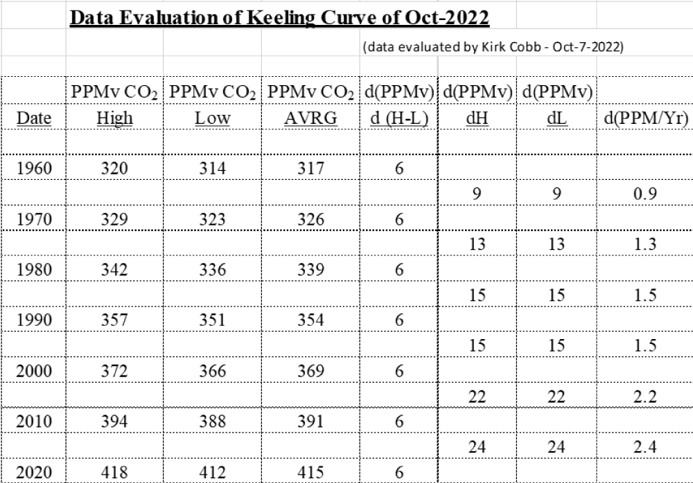
Table 3:
Biogenic carbon cycle – annual mass
The above data in Table 3, is a summary, looking at the change in atmospheric CO2 from decade to decade, from 1960 to 2020. The “high” and “low” for each year are noted; the differential from high to low each year is recorded, and within the ability to read (eye-ball) the data, the biogenic carbon cycle is consistent, not only from year to year but from decade to decade. What might be the mass of the biogenic CO2 entering and leaving the atmosphere each year, and causing this +/- 6 PPMv increase and decrease? Knowing this change in concentration, and the mass of the total atmosphere, we can calculate the magnitude of this oscillating biogenic carbon dioxide cycle:
6 PPMv x (44/28.956) x 5,150,000 GT’s / 1,000,000 = 46.95 GT’s / year = Biogenic CO2 Cycle.
(Within a reasonable margin of error, the Biogenic CO2 mass balance will be rounded to 47 GT/year.)
While reviewing online data for this paper, the author independently observed this seasonal +/- 6 PPMv cycle. As further confirmation, this recent reference from the internet was later found [10].
“The Keeling Curve also shows a cyclic variation of about 6 ppmv each year corresponding to the seasonal change in the uptake of CO2 by the world's land vegetation. Most of this vegetation is in the Northern hemisphere where most of the land is located. From a maximum in May, the level decreases during the northern spring and summer as new plant growth takes CO2 out of the atmosphere through photosynthesis. After reaching a minimum in September, the level rises again in the northern fall and winter as plants and leaves die off and decay, releasing CO2 back into the atmosphere” [10].
But, keep in mind, the biogenic carbon cycle, not only includes the oscillation of CO2 in and out of plant growth, but also the animals and people, who eat those plants, and through their respiration, exhale the CO2 after digesting the plants they eat. We cannot “double-count” this consumption of plants; the plants are either eaten or digested back to Atm. CO2, or simply dry up, die, and decompose at the end of the growing season, with CO2 returning to the Atmosphere. Either way, all of these manifestations of photosynthesis and the disposition of the carbon involved are all part of the same, seasonal biogenic carbon cycle.
Fossil fuel emissions – annual mass
However, look again at the above Keeling Curve graphs. In addition to the seasonal cycles, the graph of the CO2 concentrations continues to go higher and higher, year after year! What is causing this rise of CO2 in the Earth’s atmosphere? Can the use of fossil fuels be connected to this rise? Note the last data column in Table 3: from 1960 to 1970 CO2 concentration rose 0.9 ppm/year; from 1970 to 1980 the rise was 1.3 ppm/year; from 2010 to 2020 the rise was 2.4 ppm/year. Not only is CO2 rising each decade, but the rate of rising is also increasing. This is simply a straightforward analysis of the data from the Keeling Curve.
Let’s look at the fossil fuel consumption and emission data and compare it to the rise of CO2 in our atmosphere. Could CO2 emissions from fossil fuels contribute as much as 10%, 50%, or 90% of the total rise of CO2 in the atmosphere? What is the ratio of the annual fossil fuel emissions, to the annual rise of CO2 in our atmosphere? Let’s find out!
The “Global Carbon Project” (GCP)
The chart below was available from the “Global Carbon Project” website in 2017: [11] The GCP website has since been re-formatted, and the data are not as accessible (in 2022) as they were in 2017. The Global Carbon Project (GCP) was established in 2001, according to Wikipedia. The main object of the group has been to fully understand the carbon cycle. The project has brought together emissions experts, earth scientists, and economists to tackle the problem of rising concentrations of greenhouse gases. Its Executive Director (as of 2017?) was Josep Canadell of Australia's Commonwealth Scientific and Industrial Research Organisation (CSIRO). The GCP has additional international offices in Tsukuba, Japan, and Seoul, Korea, and an international scientific steering committee consisting of a dozen scientists from five continents. The above text is from the following source [12]:
How much CO2 is being added each year from the burning of fossil fuels? [11]
(Graph 4) The GCP appears to be a reputable organization; it is assumed that the data they present is based on valid sources of information. On that basis, the total, worldwide carbon dioxide emissions from all fossil fuels (coal, petroleum, and natural gas) are assumed to be represented in the above chart. Reading (eyeballing) from the above chart, the following gigatonnes of CO2 emissions per year, from all fossil fuel burning, are inferred:
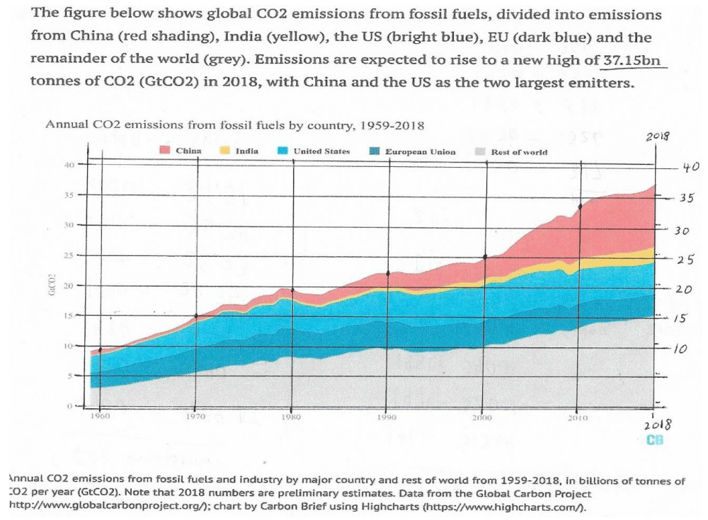
Graph 4: Global Carbon Project..
1960: 9.5 GT;
1970: 15.0 GT;
1980: 19.5 GT;
1990: 22.5 GT;
2000: 25.0 GT;
2010: 33.0 GT;
2018: 37.0 GT.
As an alternate reference for fossil fuel CO2 emissions, the site: [13] offers the following data. Each data point was read from an online interactive chart, where the cursor from your computer mouse can slide across the chart to read the CO2 GT for each year. From this interactive chart, the following data were taken. These additional notes were included on the website:
Annual CO2 Emissions:
Carbon dioxide (CO2) emissions from fossil fuels and industry. Land use change is not included.
“Our-World-In-Data” is a project of the Global Change Data Lab, a registered charity in England and Wales.
For reference, and to compare to the “GCP” data above, the data below also included 36.65 GT of CO2 emissions for 2018. By comparing the “GCP” data above, and the “ourworldindata” below, these two data sets are very similar. Therefore, for convenience, the “ourworldindata” information will be used as the reference for fossil fuel CO2 emissions in this paper, since it includes a data point for 2020 [13] (Graph 5).
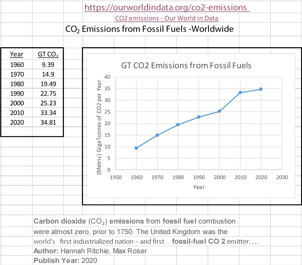
Graph 5:
All the above data will now be compiled into a single spreadsheet, shown below as Table 4 which summarizes all the information for comparison.
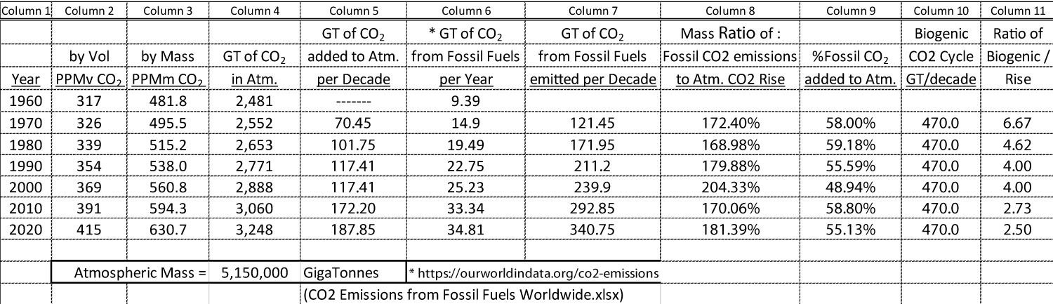
Table 4:
The data in the spreadsheet above, are a compilation of all the information, thus far, in this paper:
Column 1 – years, by decade;
Column 2 – average Atm.CO2 PPMv by volume from the Keeling Curve;
Column 3 – Atm.CO2 PPMm by mass; converted by multiplying PPMv x (44/28.956);
Column 4 = GT of CO2 in the atmosphere each decade; this column shows how the total CO2 in the atmosphere is going up each decade; = PPMm x total atmospheric mass of 5,150,000 GT.
Column 5 = the amount of CO2 that had been added to the atmosphere during the previous decade, based on the differences from the totals shown in column 4;
Column 6 = the annual fossil fuel CO2 emissions from the “ourworldindata, org”; (and similar to data from the “Global Carbon Project”).
Column 7 - data was calculated by taking the average from each decade in column 6 and multiplying by 10 to estimate the actual CO2 fossil fuel emissions generated during the previous decade, GT/decade.
Column 8 – the Ratio of data in Col.7 / Col.5 = (GT CO2 from fossil fuel emissions each decade) / (the rise in GT of CO2 in the atmosphere during each past decade). From this data, it appears that the CO2 emissions from the burning of fossil fuels more than account for ALL the rise of CO2 in the atmosphere, every decade. If this data analysis is correct, the fossil fuel emissions, alone, maybe driven ALL the rise of CO2 in the atmosphere for the past 6 decades, from 1960 to 2020. So, the excess CO2 is being absorbed into the oceans, or into caustic rock geology on land.
Column 9 – In essence, this is the reverse of Column 8; these data show what % of the fossil fuel CO2 emissions are actually being added to the atmosphere; the balance of the fossil emissions must be mostly absorbed into the oceans, or into land masses.
Column 10 – This data simply shows the simultaneous “Biogenic CO2 Cycle, which is ~ 47 GT’s/year, so over one decade, the Biogenic CO2 Cycle would release and re-absorb an estimated ~ 470 GT’s/decade. This data indicates that the biogenic CO2 cycle has always been larger than the annual growth of CO2 in the atmosphere, and larger than emissions from fossil fuels. But from 2010 to 2020, with fossil fuels dumping 340 GT/decade into the atmosphere, it is beginning to rival the natural biogenic cycle of 470 GT/decade.
Column 11 – This data shows how large the biogenic carbon cycle is, compared to the rise of CO2 in the atmosphere. As the data show, from 1960 to 1970, the biogenic carbon cycle was more than 6 times larger than the rise of CO2 in the atmosphere. From 1980 to 1990, the biogenic carbon cycle was 4 times larger than the rise of atmospheric CO2. From 2010 to 2020, the biogenic carbon cycle was still 2.5 times larger than the atmospheric rise of CO2. Over the years, the biogenic carbon cycle has remained essentially stable, but the increased dumping of CO2 from fossil fuel use has continued to grow. But from 2010 to 2020, with fossil fuels dumping 340 GT/decade into the atmosphere, it is beginning to rival the natural biogenic cycle of ~ 470 GT/decade.
Over 70% of planet Earth is covered with water and CO2 is slightly soluble in water. When CO2 dissolves in water, it forms a weak acid: CO2 + H2O ------- > H2CO3 which can ionize to H+ + HCO3- (also known as “carbonated water”). The H+ is a slightly acidic hydrogen ion that causes the pH of the ocean water to drop slightly and become more acidic. Oceanographers are concerned about this effect, the acidification of the oceans, as it jeopardizes aquatic life, such as coral reefs, and all marine life, the world over.
Comparing fossil fuel versus volcano generated CO2
Mount Pinatubo, Philippines, June 12, 1991-U.S. Geological Survey Credit: Lyn Topinka, courtesy U.S. Geological Survey.
The rise in carbon dioxide concentration in our atmosphere could be attributed to natural gaseous emissions of volcanoes, from around the world. Since volcanic eruptions can be such massive events and are prevalent the world over, it was thought at one time that volcanic activity could dwarf carbon dioxide emissions from the human use of fossil fuels.
As referenced from a recent USGS (United States Geological Survey) report online: “Volcanologists have been interested in CO2 release from volcanoes for years and have been working to improve estimates on the amount of CO2 entering the atmosphere and oceans by volcanic processes. Gas studies at volcanoes worldwide have helped volcanologists tally up a global volcanic CO2 budget in the same way that nations around the globe have cooperated to determine how much CO2 is released by human activity through the burning of fossil fuels. *Global estimates of the annual present-day CO2 output of the Earth’s degassing subaerial and submarine volcanoes range from 0.13 to 0.44 billion metric tons (gigatons) per year [14].
These volcanic CO2 emission estimates are about 1% or less, of current fossil fuel CO2 emissions of 30 to 35 gigatons/year. If large amounts of CO2 were emitted from volcanoes or other sources, the CO2 trend data on the Keeling Curve would show large “spikes” or step-wise changes of CO2 concentrations entering the global data. But the CO2 seasonal data on the Keeling Curve show NO records of any large spikes or stepwise changes of CO2 emissions – not from volcanoes, and not from massive burn-offs of biomass.
How about other sources of biogenic carbon?
The Biogenic CO2 data in the Keeling Curve, are very consistent, year after year; emissions of “biogenic” carbon dioxide appear to have minimal impact on the CO2 historical “rising trend” data.
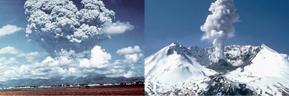
Ruminant animals, such as cows, goats, sheep, deer, elk, moose, bison, water buffalo, caribou, camels, giraffes, and antelope, have all been eating plants for hundreds of thousands of years, and their anaerobic stomachs have emitted carbon dioxide and methane. But none of these biogenic carbon sources appear to be contributing to rising atmospheric carbon. It would seem logical, if the human population across planet Earth, systematically burned massive amounts of forests and other living biomass, the Keeling Curve data trends would eventually see spikes, or stepwise jumps, in CO2 concentrations. But there simply are no records of any of these massive dumps of biogenic carbon into the atmosphere. Likewise, growing and decaying biomass in saltwater marshes and freshwater swamps the world over, anaerobically generate CO2 and CH4, but show no measurable effect. Plants (and animals) grow in swamps and marshes during the growing season and convert CO2 and water to biomass. When these biomass sources die and anaerobically decay, the biomass is converted back to biogenic CO2 and CH4 and returns to the atmosphere, ready for another photosynthetic cycle [15].
CLEAR center
“Clarity and Leadership for Environmental Awareness and Research” - at UC Davis.
The Biogenic Carbon Cycle and Cattle
February 19, 2020, By Samantha Werth, Ph. D., UC Davis
An excerpt from Dr. Werth’s article:
Cattle - belch methane (CH4), a greenhouse gas - but it is part of the biogenic carbon cycle.
Photosynthesis – plants convert Atm. CO2 to cellulose; ruminants eat cellulose, and convert a portion to Methane. After ten years the methane is broken down and converted back to Atm. CO2. The cycle begins once again. Methane belched from cattle (and all ruminants) is not adding new carbon to the atmosphere. Rather it is part of the natural cycling of carbon through the Biogenic Carbon Cycle.
Fossil Fuels Are Not Part of the Biogenic Carbon Cycle. It takes 1,000 years or more, for CO2 released from the burning of fossil fuels to be redeposited and thus has a longstanding impact on our climate, unlike the short-term biogenic carbon cycle.
As noted by the researchers at UC-Davis, all “emissions” from ruminants, as well as food wastes in landfills, and decaying biomass in swamps and marshes, are just different chapters of the same story. In all these cases, the carbon source is CO2 from the atmosphere. Photosynthesis converts the CO2 to biomass, be it plants, animals that eat plants, or each other. Eventually, the biomass, including plant and animal biomass, dies and decomposes and the carbon is returned to the atmosphere, either as CO2 directly, or as methane, which converts back to CO2 in just a few years. There is no net increase in the mass of carbon in the carbon cycle system. But, if we continue to dig up and burn carbon, in the form of coal, petroleum, or natural gas, these fossil sources are being added to the system, and driving CO2 concentrations up, in the atmosphere – that is what is driving global warming, due to tri-atomic CO2 which absorbs low-frequency infrared radiation, causing the planet to warm.
The methane cycle
A great deal of attention is currently being addressed to understanding the role that methane plays in global warming. Several references are noted below, to help clarify this topic.
From the UC-Davis “CLEAR Center” [16]:
For example, CO2, a long-lived gas, takes hundreds of years to break down in the atmosphere and as a result, collects in the atmosphere………. Methane, on the other hand, is a short-lived gas and breaks down in about ten years….. to become CO2 and water vapor……..
First of all, biogenic methane, and the CO2 that it becomes, are part of the biogenic carbon cycle. Occurring already for thousands of years, the biogenic carbon cycle sees atmospheric carbon sequestered by plants and transformed into carbohydrates. Those carbohydrates are fed/eaten by animals like cattle and then emitted as methane and CO2 again through respiration. Then the cycle restarts. On the other hand, CO2 emitted through the burning of fossil fuels (i.e. oil and coal) adds more than normal quantities, that have been trapped underground for thousands of years.
The excerpts below, are from the US-EPA website noted here [17].
The Global Warming Potential (GWP) was developed to allow comparisons of the global warming impacts of different gases. Specifically, it is a measure of how much energy the emissions of 1 ton of a gas will absorb over a given period of time, relative to the emissions of 1 ton of carbon dioxide (CO2). ……………
By definition, CO2 has a GWP of 1 regardless of the time period used, because it is the gas being used as the reference………
For example, for CH4, which has a short lifetime, the 100-year GWP of 27–30, is much less than its 20-year GWP of 81–83……..
Methane (CH4) is estimated to have a GWP of 27-30 over 100 years. CH4 emitted today lasts about a decade on average, which is much less time than CO2. But CH4 also absorbs much more energy than CO2. The net effect of the shorter lifetime and higher energy absorption is reflected in the GWP…….
Methane has a significant energy absorption tendency; but remember, the actual total, energy absorption is directly related to its presence in the atmosphere. So, the total GWP of CO2 and CH4 are both proportional to their concentrations in the atmosphere. So, let’s compare the current “mass” of methane in our atmosphere, to the current “mass” of carbon dioxide in our atmosphere. From Table 1, the current CO2 PPMm = 630.61; the current CH4 PPMm = 0.94. Now, let’s compare the total GWP of each gas, CO2 and CH4, based on their actual presence in the atmosphere, by multiplying the concentration of each of these gases, by their assigned GWP (global warming potential):
Carbon dioxide GWP = 630.61 x 1 = 630.61; the methane GWP = 0.94 x 30 = 28.2. So, we can estimate the ratio of the CO2-GWP to the CH4-GWP to be: 630.61 / 28.2 = 22.36; in other words, the current CO2 in our atmosphere has 22.36 times as much warming effect, as the current methane in our atmosphere. Yes, pound for pound, methane is a much more potent GHG (greenhouse gas). But methane’s presence in the atmosphere is much less than carbon dioxide, and methane remains in the atmosphere for a very short amount of time, compared to carbon dioxide. Within a few years, methane is converted back to carbon dioxide (and water).
As noted earlier in this paper, the UC-Davis CLEAR Center points out that “biogenic” methane is simply part of the larger “biogenic carbon cycle”; it continues to cycle through the system but does not contribute any increase of new carbon into the atmosphere. This is true, not only for ruminant animal emissions, but also for food wastes in landfills, and “swamp gas” from freshwater swamps and saltwater marshes, the world over. These are all part of the natural biogenic carbon cycle. And the oscillating seasonal cycles of carbon dioxide shown on the Keeling Curve of Graph 2 in this paper, indicate a very consistent biogenic cycle year after year, and decade after decade.
But, the US EPA is becoming more concerned about “fossil” based methane emissions from oil and gas wells [18].
CLIMATE: Biden to announce tougher regulations on methane emissions from oil and gas production, published Tuesday, Nov-2-2021 - CNBC
The Environmental Protection Agency on Tuesday (11-2-2021) proposed rules to plug methane gas leaks at hundreds of thousands of oil and gas wells in the U.S., marking its most aggressive action yet to curb climate-warming greenhouse gas emissions. The agency’s measures will strengthen regulations on new oil and gas wells, and impose new requirements for existing wells that previously escaped methane regulations [19].
Methane concentration at NOAA's Mauna Loa observatory thru July 2021:
A record-high of 1912 ppb was reached in December 2020 (Graph 6).
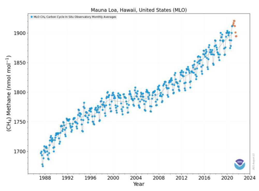
Graph 6:
An additional internet reference estimates that methane concentrations in the atmosphere, have historically been about 700 parts per billion, and reached 900 ppb by 1900, and 1,000 ppb by 1930. But during the latter half of the 20th Century methane levels have grown rapidly, primarily due to increasing industrial activity, particularly, oil and gas exploration. As shown in the above graph, the NOAA Mauna Loa, Hawaii data now indicate methane levels approaching 2,000 ppb or 2 PPMv.
The United Nations has warned the world that methane emissions must be reduced asap [20].
Published Thursday, May 6 2021-CNBC: A landmark United Nations report has declared that drastically cutting emissions of methane, a key component of natural gas, is necessary to avoid the worst impacts of global climate change. “Cutting methane is the strongest lever we have to slow climate change over the next 25 years and complements necessary efforts to reduce carbon dioxide,” Inger Andersen, executive director of the U.N. Environment Programme, said in a statement. “The benefits to society, economies, and the environment are numerous and far outweigh the cost,” Andersen said. “We need international cooperation to urgently reduce methane emissions as much as possible this decade.” The fossil fuel industry has the greatest potential for reducing global emissions at little or negative cost, by repairing leaks from oil and gas infrastructure, the report said. It added that companies that prevent leaks and capture methane could profit while curbing methane release.
Another potential threat from methane emissions comes from the Arctic permafrost region [21].
"The mechanism of abrupt thaw and thermokarst lake formation matters a lot for the permafrost-carbon feedback this century," said first author Katey Walter Anthony at the University of Alaska, Fairbanks, who led the project that was part of NASA’s Arctic-Boreal Vulnerability Experiment, a ten-year program to understand climate change effects on the Arctic. "We don’t have to wait 200 or 300 years to get these large releases of permafrost carbon. Within my lifetime and my children’s lifetime, it should be ramping up. It’s already happening but it’s not happening at a really fast rate right now, but within a few decades, it should peak."
There are many aspects of the methane story, which are still being evaluated. But, we know that biogenic methane has been generated, and cycled through the biogenic carbon cycle, from ruminants, and seasonal anaerobic emissions from swamps and marshes, with little or no major impact on climate change for thousands of years. But during the 20th Century, with increased industrialization, oil and gas exploration, and methane gas leaks from infrastructure, these sources of methane, while short-lived in the atmosphere, are quickly converted to CO2, and contribute additional fossil-based carbon to the environment. And, as the world is already beginning to warm, the growing threat of sequestered methane (and CO2) in the Arctic permafrost region, has become an additional concern. With all of these aspects, the role of methane in the climate change saga, cannot be ignored.
Fossil fuel burning more than accounts for all the rise of CO2 in the Atmosphere; the balance must be absorbed in the oceans and on land. Therefore, CO2 from fossil fuel burning is the primary (or only) source driving UP Atmospheric CO2.
The annual, seasonal biogenic CO2 cycle is very consistent over many years, even decades, and does not appear to be the major driving force for the rise of CO2 in the Atmosphere. There are NO major spikes or stepwise jumps in the Keeling Curve trend data due to volcano emissions or massive biomass burn-offs.
Trying to solve “Climate Change” by addressing biogenic carbon emissions – is a useless distraction from the REAL PROBLEM – the burning of fossil carbon.
Methane from Cows? Biogenic carbon! Eat Meat? Biogenic carbon! These have minimal, or NO effect on Climate Change. The atmospheric data record is clear. Stop creating problems to solve that don’t exist, such as methane emissions from ruminants! These are only distractions from the real problem, the burning of fossil fuels.
Replacing the use of fossil fuels with biofuels made from biogenic carbon is the basis for the “renewable fuels” industry. Stop using fossil carbon and instead use biomass for fuels, which are carbon neutral. It is important to understand the difference between Fossil Carbon and Biogenic Carbon! The wood pellet industry is an attempt to replace coal (a fossil fuel) with a biogenic source (wood) for home heating and electrical power generation. Food wastes can be used, either in landfills or industrial anaerobic digesters, to generate “renewable natural gas” (RNG), in an attempt to replace fossil-based natural gas.
As carbon dioxide increases in our atmosphere, the behavior of the molecular physics of this tri-atomic gas will slowly increase the absorption of the infrared radiation trying to escape Earth’s atmosphere back out into space and cause the Earth to warm ever so slightly.
As Earth warms, the oceans, which cover over 70% of this planet, will also warm slightly, thus the vapor pressure of water will increase slightly, and thus slightly increase the volume of water vapor (also a tri-atomic gas) in our atmosphere. This “positive feedback” effect will contribute just a bit more absorption of a bit more infrared radiation, trying to escape Earth’s atmosphere. And so, the Earth slowly warms.
More water vapor in our atmosphere will cause heavier rain storms, heavier snow storms, and more flooding in more places.
The warming atmosphere will cause more mountain and polar glaciers to melt, adding to ocean volumes.
The warming of the oceans will cause water density to decrease slightly, thus slightly expanding the volume of the oceans and compound, even more, ocean levels rising.
Eventually, coastal cities around the world may become flooded by the rising seas and may become uninhabitable.
Some of the increasing levels of carbon dioxide will dissolve in the oceans, causing them to become slightly more acidic, and disrupt the lifecycle of aquatic ecosystems.
Data indicate that volcanoes are not a primary contributor to rising atmospheric carbon dioxide levels; in fact, volcanoes are estimated to contribute less than 1% of the rise.
The management of biomass for agriculture and forestry around the world may contribute to the overall carbon imbalance. But seasonal carbon dioxide variations in the atmosphere, as shown on the Keeling Curve, do not indicate biomass management as a significant impact to date. That does not mean that the future management of biomass is unimportant.
The overall mass balance of fossil fuel emissions, shown in Table 4, is very compelling! It can only be hoped that the sources of data used to construct Table 4 are wrong! Please, someone, identify that the evaluation of these data is in error.
If not, then fossil fuel emissions are contributing nearly 2 times as much carbon dioxide as is being added to the atmosphere each year. The excess balance of carbon dioxide must be added to the oceans and landmasses. At what point do these other “carbon sinks” become saturated, and the rise in CO2 in the atmosphere accelerates even faster?
It has been reported that sequestered carbon, buried in arctic permafrost, is beginning to melt, and may also add to the atmospheric carbon balance (CO2 and CH4). This adds an additional threat to global warming.
It has also been reported that analytical chemists are trying to evaluate carbon isotopes (C12, C14) to determine if some of the rises of atmospheric CO2 are biogenic, rather than fossil carbon. Could human agriculture be contributing to the rise? Even so, the mass balance, as indicated in this paper in Table 4, if it is correct, shows overwhelming evidence that fossil fuel emissions are the main (or only) driver of climate change. Agriculture, it appears, cannot be blamed for climate change. The fossil fuels used to operate agricultural machinery can be blamed for climate change, but not the biogenic carbon of plant growth.
Atmospheric scientists, Earth scientists, geologists, physicists, geo-chemists, biologists, and oceanographers, have studied in great detail, the consequences of the continuing rise of carbon dioxide in our atmosphere and oceans. There is much to learn, but much has been learned. And with this knowledge, we also have a growing responsibility to care for planet Earth. We hold this responsibility not only for future generations of people, but for all plants and animals, with which we share this planet, and call it home.
If we allow the planet to continue to warm, causing more flooding events around the world, and also more intense droughts, disruption of agricultural production cannot be avoided. As the world population continues to grow, mass starvation could return to the world, as the number of people increases, and as agriculture begins to fail.
The goal of this paper was not meant to answer all the questions that can be raised regarding climate change, but to establish some of the basic science needed to help understand this unfolding world event. In particular, it was the goal of this retired process engineer, to try to make sense of the current “mass balance” of the fossil fuel CO2 emissions being added to our atmosphere each year. Do these emissions contribute 10%, 50%, or 90% of the rise of CO2 in the atmosphere? That question seems to be answered! Fossil fuel emissions are providing over 170% of the CO2 being added to the atmosphere. From this simple “mass balance” perspective, the fossil fuel CO2 emissions, more than account for ALL of the rise of CO2! Without fossil fuel emissions, the biogenic seasonal cycle would certainly continue but may cause a NO rise in CO2. It has been said many times in the past few years, that we have all the technologies needed to address the growing concerns about the rising carbon dioxide in our biosphere; we simply need to find the political will to rise to these challenges. Energy corporations that have made their fortunes in the past 100 years, can continue to be the “energy” suppliers of the future if they so choose, but they need to leave the fossil carbon in the ground, and embrace renewable, sustainable resources, and technologies that are available today. And, those corporations have the financial, technical, and managerial resources needed to make this transition, if they so choose. As human societies around the world embrace this new direction, local citizens need to understand that the energy sector transition may cost more during that transition. But as new technologies become the norm, costs will come down, as in every other transition that we have made in the past few centuries.
Does world population have a role in climate change?
As people the world over strive for better living conditions for themselves, it is important to recognize that unlimited growth of the human population can also contribute to the growing challenge. It was quite surprising, when constructing the graph below, the apparent relationship of the gigatonnes of CO2 emissions from fossil fuels, to the rise of the human population, from 1960 to 2020. There has clearly been a linear correlation during the past 60 years, as can be seen in Graph 7.
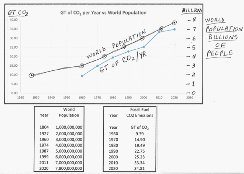
Graph 7: Fossil Fuel CO2 emissions from “ourworldindata”.
World Population data [22].
Part of our responsibility as human beings is to recognize that we must control, not only our consumption of resources but also the size of our population. Human beings are part of this planet Earth, no less than the trees and grass and flowers, and animals with which we share it. Sooner or later, we need to learn how to live sustainably in this magnificent, but finite, home. The sooner we can convert our energy technologies away from fossil-based fuels, and convert to renewable energy, including solar, wind, and biogenic-based fuels, the brighter will be the future for the generations to come.
Estimate of annual biogenic CO2 from human respiration
One more table of data is offered below, which may be of interest, along with the human population’s impact on climate change. Photosynthesis has been discussed somewhat, in this paper. It is important to keep in mind that this natural process, is the basis of the total food supply chain for all living beings on planet Earth. Photosynthesis does not only generate large amounts of cellulosic biomass, but also generates all the starches and sugars (carbohydrates), vegetable oils, and plant-based proteins, which sustain all animal life on the planet, including humans. As with all animals, humans consume these starches (or carbohydrates), vegetable oils, and proteins to meet all of our nutritional requirements, and then discharge much of that biogenic biomass, via our respiration. Assuming an average metabolic energy rate of ~ 2,500 kilocalories per person per day, the Table 5 below estimates the amount of carbon dioxide emitted by all humans on planet Earth each year. Note that this human respiration is, in fact, a small portion of the annual biogenic carbon cycle, which has been estimated to be ~ 47 GT/year.
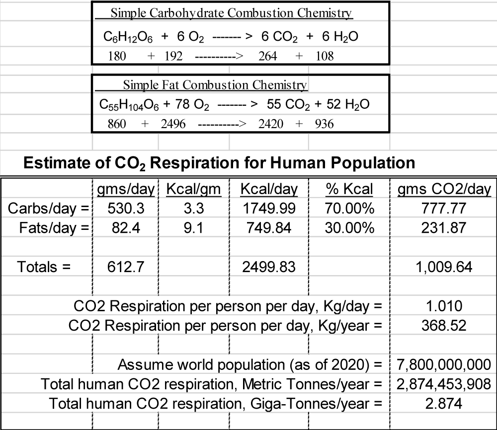
Table 5:
From the figures above, it can be estimated that total worldwide, human respiration accounts for (2.9/47 =) 6.17% of the total biogenic carbon dioxide cycle. Recall that the 47 GT/year figure is an estimate, from the Keeling Curve seasonal oscillation “differential” between the opposing Northern and Southern Hemispheres’ biogenic CO2 cycles. The total, combined biogenic cycles of the Northern + Southern Hemispheres is not known, at least from the data presented thus far in this paper. However, if these opposing biogenic cycles were proportional to their respective land masses (68% north; 32% south) then the “total” annual biogenic cycle could be estimated to be: 0.68X - .032X = 47 GT; thus “X” = total CO2 biogenic annual cycle might be estimated to be: “X” = 130 GT of CO2. Then, total Northern = 88.4 GT/year and Southern = 41.6 GT/year. The total = 88.4 + 41.6 = 130.55 GT/year, and the difference, the North-South = 88.77 – 41.77 = 47.0 GT/year. Let’s compare this estimated “total” biogenic CO2 cycle to an independent internet reference from [23].
Another estimate for the “Total” annual biogenic CO2
The cycling of biogenic atmospheric gases [23].
Each year, photosynthesis fixes carbon dioxide and releases 100,000 megatons of oxygen to the atmosphere.
(Not sure what the reference is, for this 100,000 megatons of oxygen. But let’s test this number).
On this basis, the annual biogenic Carbon Dioxide mass can be estimated.
The carbon cycle is fully coupled to the oxygen cycle. Each year, photosynthesis fixes carbon dioxide and releases 100,000 megatons of oxygen to the atmosphere. On a seasonal basis, an enrichment of atmospheric carbon dioxide occurs in the winter half of the year, whereas a drawdown of atmospheric carbon dioxide takes place during the summer. Note: 100,000 megatons = 100 gigatons, or 100 GT.
6 CO2 + 6 H2O ----solar energy------ > C6H12O6 + 6 O2
6 x 44 + 6 x 18 -------------------- > 180 + 6 x 32
264 + 108 --------------------- > 180 + 192
137.5 GT/Y + 56.25 GT/Y ---------- > 93.75 GT/Y + 100 GT/Y
This is very interesting, and essentially confirms the estimate above. Thus, 137.5 GT/year of CO2 was back-calculated from the assumption that an annual total of 100 GT of oxygen are liberated by photosynthesis worldwide. Independently, the differential between the Northern and Southern hemispheres, from the Keeling Curve, led to an estimated figure of 130.55 GT/year of CO2 to be the total of the Northern + Southern hemispheres of their respective biogenic CO2 cycles. These two estimates seem to confirm one another.
So, if the total annual biogenic CO2, from both hemispheres, is ~ 130 GT/year, and the total human respiration is estimated to be 2.9 GT/year, then the CO2 from human respiration is actually ~ (2.9/130 = ) 2.2% of the total CO2 biogenic cycle. It is hoped that the reader of this paper, finds this little calculation to be as interesting as the author found it to be.
- Recent update of atmospheric composition from the NASA Earth Fact Sheet. https://nssdc.gsfc.nasa.gov/planetary/factsheet/earthfact.html
- Historical NASA CO2 data. https://data.giss.nasa.gov/modelforce/ghgases/Fig1A.ext.txt
- Reference to atmospheric pressure. www.aqua-calc.com/what-is/pressure/atmosphere
- Basic geometry of planet Earth. https://nssdc.gsfc.nasa.gov/planetary/factsheet/earthfact.html
- https://en.wikipedia.org/wiki/Atmosphere_of_Earth#:~:text=The%20atmosphere;
- https://www.bing.com/search?q=mass+of+the+atmosphere+in+kg&form;
References for the mass of Earth’s atmosphere.https://www.britannica.com/story/how-much-does-earths-atmosphere-weigh - Biography of Charles David Keeling. https://scrippsco2.ucsd.edu/history_legacy/charles_david_keeling_biography.html
- Notes regarding Charles Keeling’s career. https://wiki.alquds.edu/?query=Keeling_Curve
- The Keeling Curve, published by the “NOAA Global Monitoring Laboratory” as of October 5, 2022 – note, this referenced website includes both the full Keeling Curve from 1958 to 2022, and the excerpt curve for 2018 through 2021, and a portion of 2022. https://www.esrl.noaa.gov/gmd/ccgg/trends/index.html
- Reference to the land masses of the Northern and Southern Hemispheres. www.worldatlas.com/articles/which-hemisphere-has-the-largest-area-covered-by-land.html
- Reference to the Keeling Curve biogenic carbon cycle as 6 PPMv for each annual season. https://wiki.alquds.edu/?query=Keeling_Curve:
- Reference to the Global Carbon Project website; note, the graph shown on page 9 was available from this website in 2017, but is no longer available; this graph in 2017 had been printed and scanned, but is no longer available in 2022. http://www.globalcarbonproject.org.
- Reference to the Global Carbon Project organization. https://en.wikipedia.org/wiki/Global_Carbon_Project
- Reference for “Our World in Data”. https://ourworldindata.org/co2-emissions
- Reference to volcanic CO2 emissions from the USGS. https://volcanoes.usgs.gov/vsc/file_mngr/file-154/Gerlach-2011-EOS_AGU.pdf
- Website for the UC-Davis regarding methane emissions from cattle. https://clear.ucdavis.edu/explainers/biogenic-carbon-cycle-and-cattle
- Methane, carbon dioxide, and the biogenic carbon cycle from UC-Davis. https://clear.ucdavis.edu/explainers/gwp-star-better-way-measuring-methane-and-how-it-impacts-global-temperatures
- US-EPA and the GWP – Global Warming Potential. https://www.epa.gov/ghgemissions/understanding-global-warming-potentials
- The US-EPA gets tough on methane leaks from the oil and gas sector. https://www.cnbc.com/2021/11/02/-biden-epa-gets-tough-on-methane-leaks-from-oil-and-gas-sector-.html
- Methane atmospheric concentrations from NOAA Mauna Loa Observatory from 1988 to 2021. https://en.wikipedia.org/wiki/Atmospheric_methane
- United Nations report – world must cut methane emissions. https://www.cnbc.com/2021/05/06/world-must-cut-methane-emissions-to-avoid-worst-of-climate-change-un-says.html
- NASA report on methane permafrost emissions. https://www.nasa.gov/feature/goddard/2018/unexpected-future-boost-of-methane-possible-from-arctic-permafrost
- World population. https://www.worldometers.info/world-population/world-population-by-year/
- Estimate of total annual photosynthetic CO2 from both the Northern and Southern Hemispheres. https://www.britannica.com/science/climate